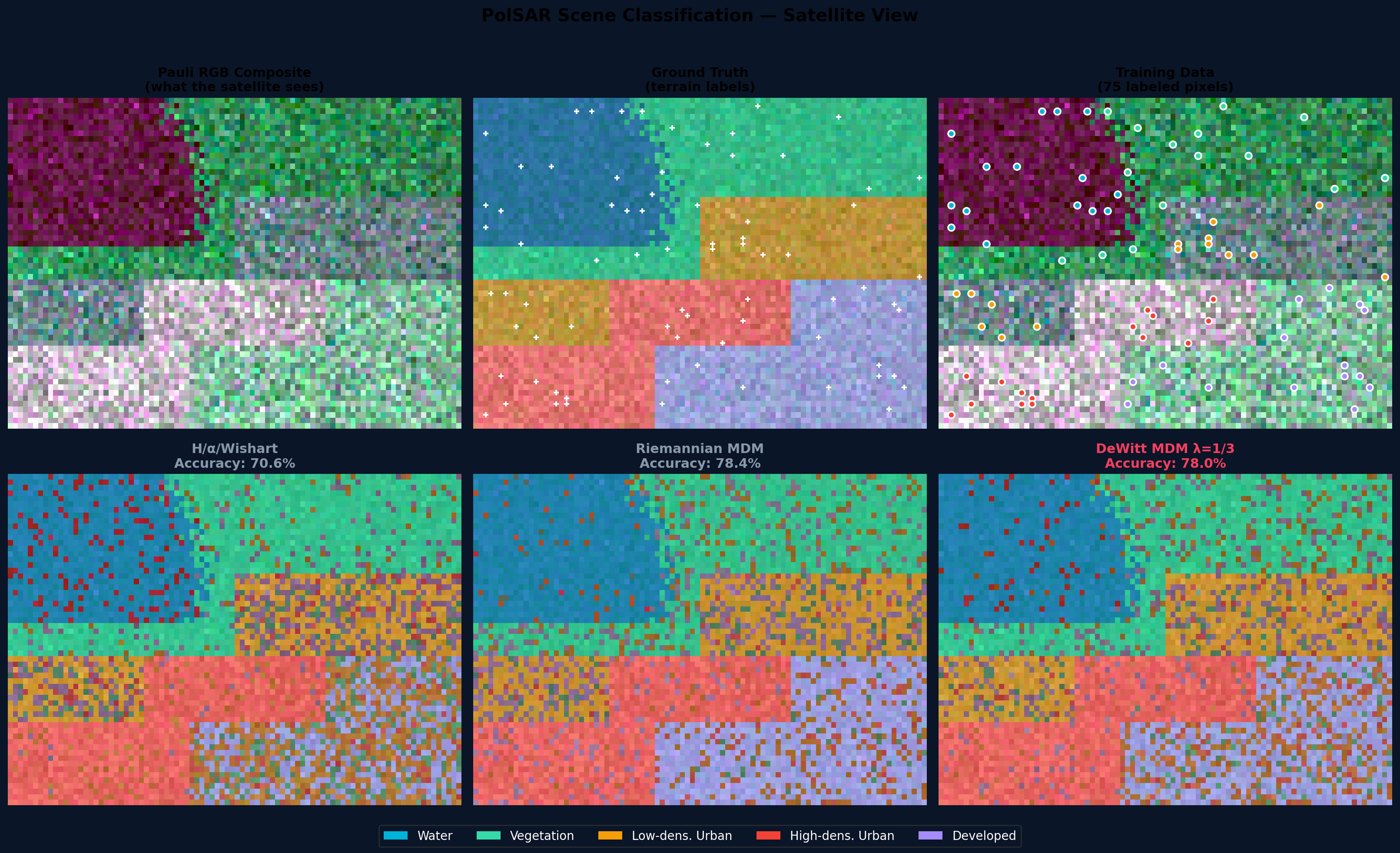
Polarimetric SAR coherency matrices are 3×3 SPD matrices on GL+(3)/SO(3). The DeWitt supermetric separates scattering mechanism from backscatter power — solving the range-dependent power variation problem that plagues standard methods.
Polarimetric SAR measures the full scattering matrix of each pixel. The resulting 3×3 coherency matrix T encodes both the scattering mechanism (surface, volume, double-bounce) and the overall backscatter power.
In real SAR imagery, identical terrain at different ranges or incidence angles produces different power levels. Standard classifiers — including H/α/Wishart and Riemannian MDM — conflate power with mechanism, reducing accuracy when labeled data is scarce.
The DeWitt metric on GL+(3)/SO(3) provides a family of Riemannian distances that separately weight the trace (power) and traceless (mechanism) components of the coherency matrix. This allows the classifier to focus on scattering mechanism while controlling sensitivity to power variation — exactly what PolSAR classification needs.
For 3×3 coherency matrices, the tangent space decomposes into:
The proprietary metric configuration downweights V− to focus the classifier on mechanism while retaining useful power information.
Left: what the SAR satellite captures (Pauli RGB composite). Right: DeWitt MDM classification from just 15 labeled pixels per class.
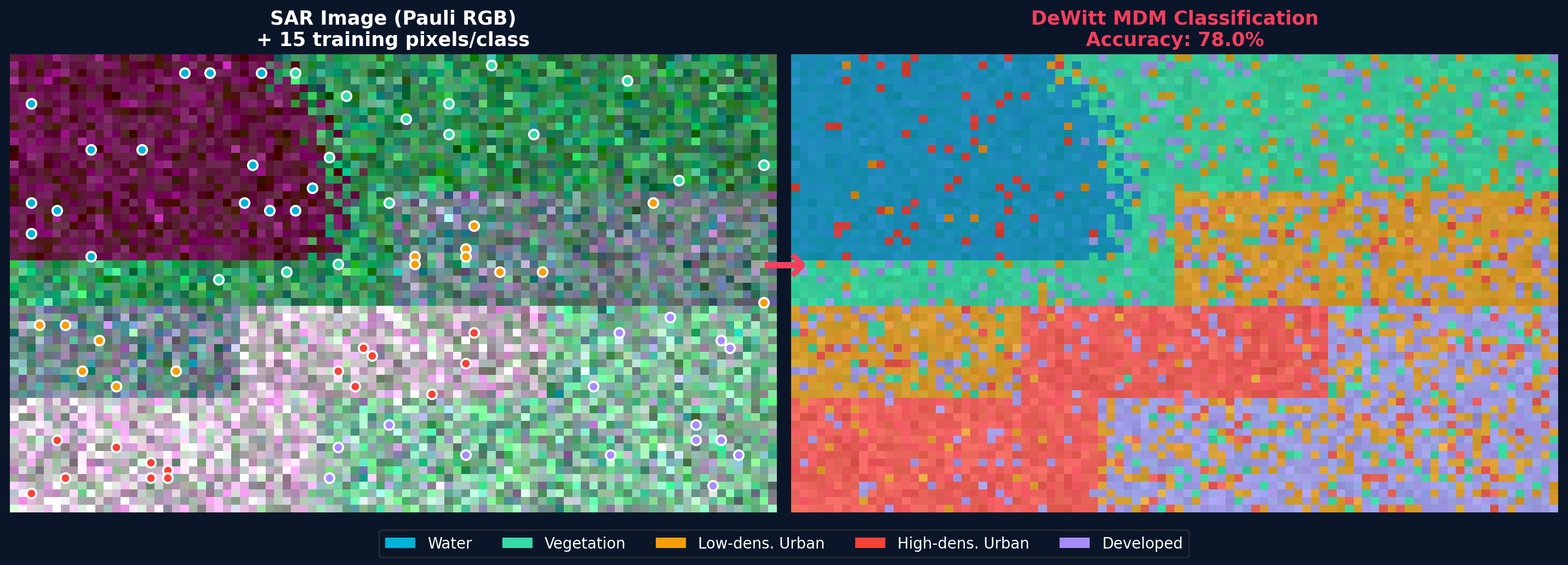
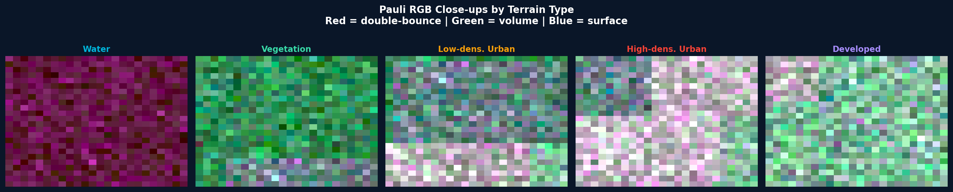
Pauli RGB: magenta = surface scattering (water), green = volume scattering (vegetation), gray/mixed = urban structures.
Each terrain type has a distinct radar signature. Water reflects away (dark/magenta), vegetation scatters volumetrically (green), urban structures create strong double-bounce returns.
AIRSAR San Francisco (L-band, 5-class). Real data benchmark on 900×1024 scene. Full results: DOI 10.5281/zenodo.19192324
Top row: SAR image, ground truth overlay, training pixel locations. Bottom row: H/α/Wishart (76.6%), Riemannian MDM (78.4%), DeWitt MDM (78.0%).
Each pixel's 3×3 coherency matrix decomposed into V+ (scattering mechanism) and V− (backscatter power).
Row 1: Raw coherency matrix T. Row 2: V+ (traceless shape — terrain-specific). Row 3: V− (trace power — varies with range, NOT terrain-specific).
One-parameter family of metrics that interpolates between standard Riemannian and power-invariant classification.
A proprietary family of geodesic distances on GL+(3)/SO(3) controls the trade-off between scattering mechanism and backscatter power sensitivity.
The tangent space naturally decomposes into traceless (shape, 5D) and trace (power, 1D) components. This geometric structure provides the foundation for power-invariant classification.
With only 5 labeled pixels per class, geometric features achieve 79.1% accuracy (+9.3pp over raw input) — critical for rapid deployment in new terrain or disaster response scenarios.
Multiple geometric classifiers are combined through proprietary ensemble methods, achieving state-of-the-art results across all data regimes.
Same terrain at different power levels. Standard metrics cluster by power; DeWitt collapses power variation while preserving terrain separation.
Left: Standard Riemannian metric — same terrain at different power levels forms separate clusters. Right: Geometric correction — power variation collapsed, terrain classes separate cleanly.
Quantifying how much of each pixel's information is scattering mechanism (V+) vs backscatter power (V−).
Left: V+ energy (shape) separates classes vertically. V− energy (power) smears them horizontally. Right: Shape-to-total ratio per class — urban terrain has the most shape information.
How the proprietary metric reshapes the tangent space cluster structure.
Standard Riemannian metric: classes overlap due to power variation. With progressive geometric correction, terrain classes tighten into distinct clusters.
DeWitt sharpens the block-diagonal structure — same-class pixels become closer, different-class pixels stay separated.
How fast do methods degrade with limited training data? The adaptive ensemble dominates across all regimes.
5-class terrain classification. ResNet-SE, 15×15 patches, 5 seeds, 100 epochs. Real AIRSAR data.
import requests
# Classify a PolSAR coherency matrix via API
response = requests.post(
"https://api.omnisciences.io/polsar/classify",
json={
"coherency_matrix": T.tolist(), # 3x3 SPD matrix
"method": "ensemble",
"n_looks": 9,
}
)
result = response.json()
print(f"Prediction: {result['prediction']}")
# Prediction: vegetation
print(f"Confidence: {result['confidence']:.1%}")
# Confidence: 91.3%
# Batch classification for full scenes
batch = requests.post(
"https://api.omnisciences.io/polsar/classify_scene",
json={"scene": scene_matrices, "n_looks": 9}
)
print(f"Classified {batch.json()['n_pixels']} pixels")
Terrain classification, target recognition, and change detection from PolSAR covariance matrices. Few-shot capable: 5–10 labeled samples, no GPU.
Crop classification, flood damage assessment, and post-disaster mapping from SAR. Works through clouds where optical fails.
Forest type classification and deforestation detection for carbon credit verification. Change detection between SAR acquisitions.
Defense subcontracting: SAR classification pilots from $25K. Contact us